Excel Training: Custom Conditional Formatting
The goal here is to add 3 conditional formats to the following table (lesson-8b.xlsx) in order to:
- Format cells containing "x"
- Format the column of the day (based on today's date)
- Format a row (based on a search)
Formatting cells containing "x"
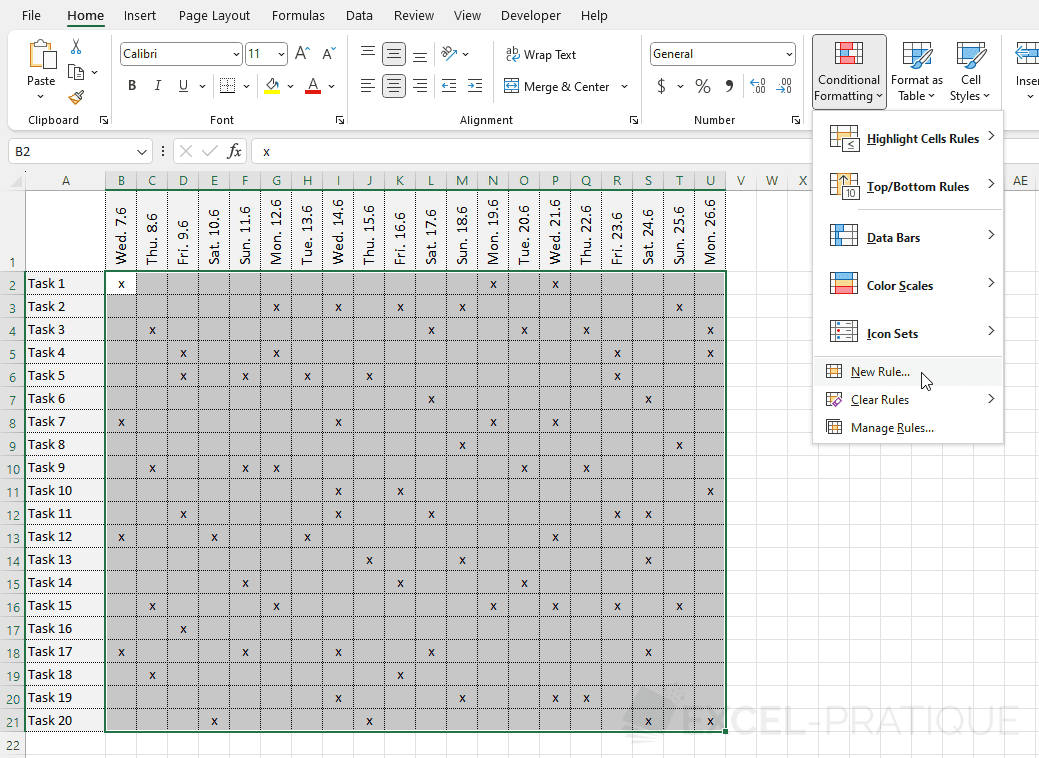
We will start by adding the first conditional format by selecting the range of cells and clicking on "New Rule" in "Conditional Formatting":
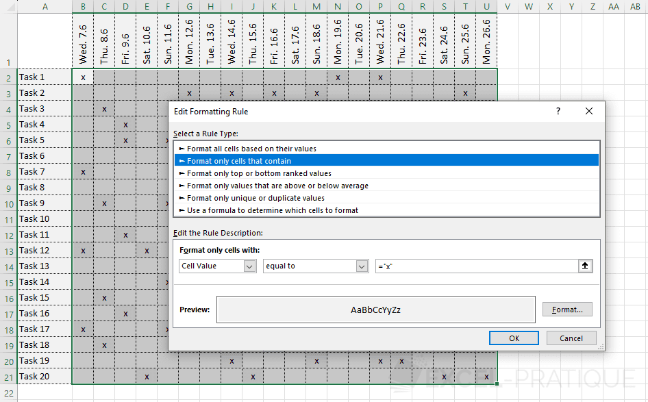
To format the cells whose value is equal to "x", choose Cell Value equal to ="x" and set a format:
Formatting the column of the day
The goal now is to format the entire column of the schedule based on today's date (knowing that row 1 contains dates and that today's date can be obtained using the TODAY function).
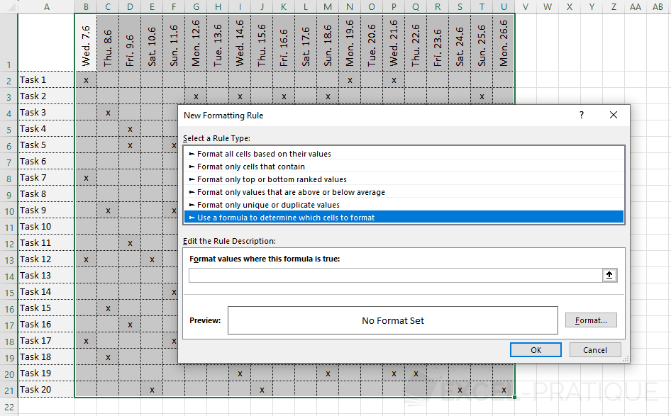
Now select the range of cells including the dates and add a new formatting rule:
Set a format then enter the formula =B1=TODAY():
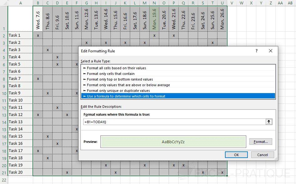
You may notice that only the cell containing today's date has been formatted.
To lock the date test to row 1, you must therefore add a $ before the 1 =B$1=TODAY():

Formatting based on a search
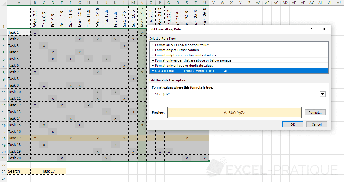
To format a row based on the search in cell B23, select the cells in the table including this time column A and add a new rule:
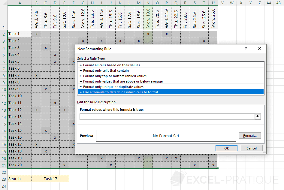
To search only in column A, you must add a $ in front of the A $A2 and 2 $ to the cell $B$23 since it must remain fixed. The formula for this conditional formatting is therefore =$A2=$B$23:
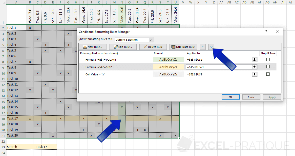
If needed, you can change the order of the different conditional formats:
Renaming a cell
Instead of entering in the formula the cell $B$23 with its 2 $, you can choose to rename this cell and directly enter its name.
To assign it a name, select cell B23, enter its new name and validate:
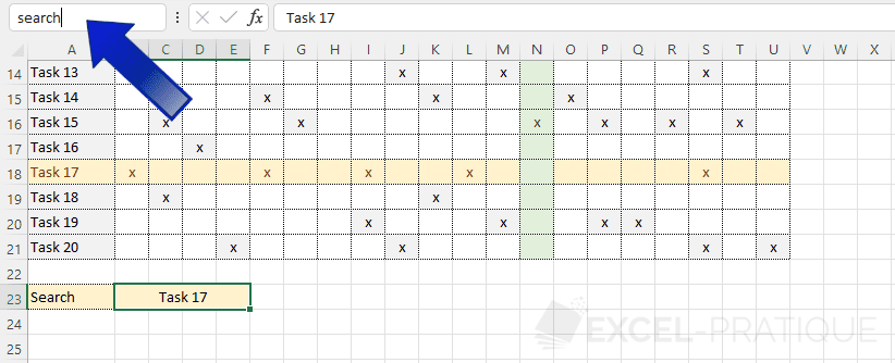
You can now enter search instead of $B$23 in the formula of the conditional format =$A2=search (or in any other formula of the workbook):
