Excel Function: HLOOKUP
The Excel function HLOOKUP searches for a value in the first row of a table and then returns the value of a cell that is in the same column as the searched value.
Usage:
=HLOOKUP(lookup_value, table_array, row_index_num, range_lookup)
Example of Use
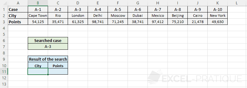
The goal here is to look up information based on the case number. The user should be able to enter the case number in the green part and then see the result of his search in the blue part:
Select the HLOOKUP function and enter:
- Lookup_value: the value to search for in the first row of the table (here, the case number)
- Table_array: the range of cells containing the table data
- Row_index_num: the row number in the table that contains the result to return (here, row 2 for the city)
- Range_lookup: FALSE or 0 to search for the exact value of Lookup_value (when in doubt, enter 0 to avoid surprises), TRUE or 1 (or leave empty) to search for the closest value to Lookup_value
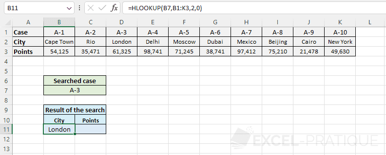
=HLOOKUP(B7,B1:K3,2,0)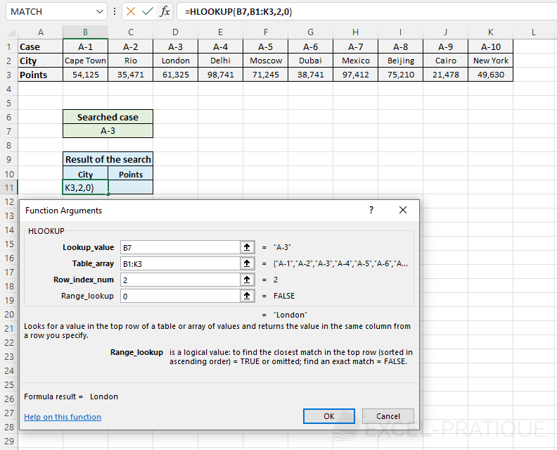
The name of the city is then displayed:
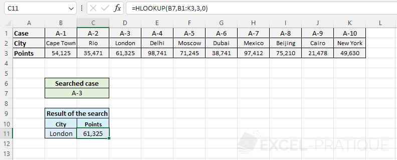
To then display the points, simply copy the formula and change the row number (replace 2 with 3):
If needed, you can download the Excel file used here: hlookup.xlsx
The HLOOKUP function searches for a value in the first row of a table, so the results cannot be above the search row. If you want to be able to search in a row that is not necessarily the first in the table, use the combination of functions INDEX + MATCH.