Excel Course: Custom Conditional Formatting

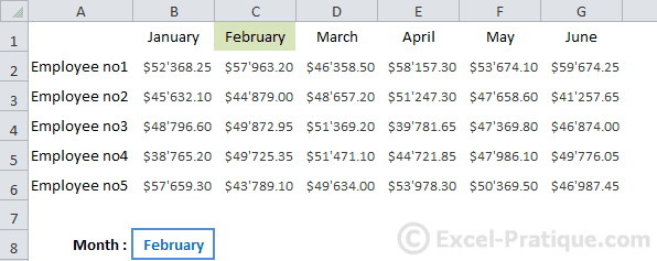
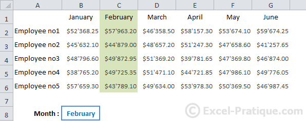
For this example, the name of a month has been entered into cell B8.

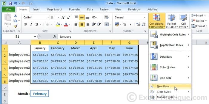
The goal here is to create a CF that can automatically shade the column in the table for the month whose name appears in B8.

Select all the cells in the table and choose "New Rule...":

Choose the last kind of rule to enter a formula.

Begin your formula with an = sign, then enter the first cell to test (in this case, B1) and finally enter =$B$8 (with the $ sign to "fix" the cell reference).

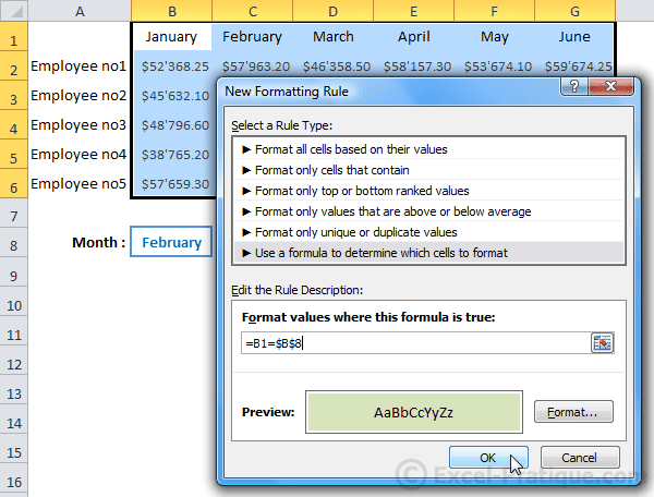
Using =B1=$B$8, the CF will be applied to every cell that contains the search value (in this case, February).

The formula =B1=$B$8 is for the first cell in the table, and will be modified for the other cells (as in a Fill Series command).

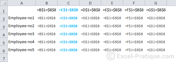
This table should help you better understand the test that is being performed on each cell:

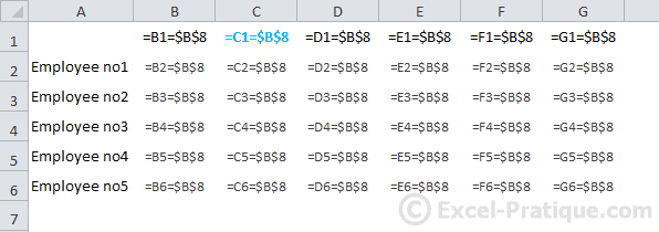
To format the entire column, rather than just a single cell, we will have to "fix" the row number using a $ sign.

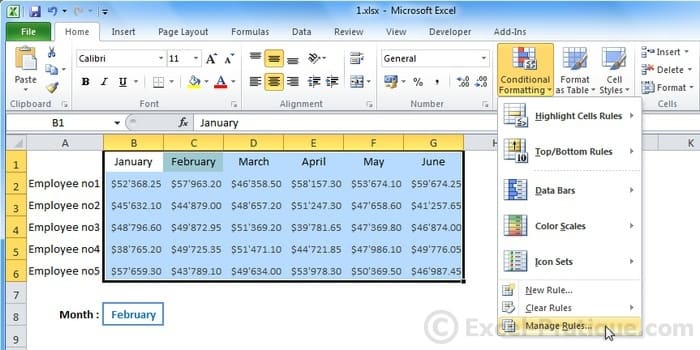
To edit the formula, click on "Manage Rules..." then "Edit the Rule...".

Add a $ before the row number.

This time, the whole column has been formatted.

The tests performed on the cells:

To format a whole column, now all we have to do is change the month that appears in cell B8.